The Day Words Became Vectors

What is word vectorization?

Word vectorization refers to a set of techniques that aims at extracting information from a text corpus and associating to each one of its word a vector. For example, we could associate the vector (1, 4, -3, 2) to the word king. This value is computed thanks to an algorithm that takes into account the word’s context. For example, if we consider a context of size 1, the information we can extract from the following sentence:

The king rules his kingdom

is a set of pairs:

(the king), (king rules), (rules his), (his kingdom)

If we now consider another sentence:

I see a king

and the associated pairs:

(I see), (see a), (a king)

We notice that we have 2 similar pairs across the 2 sets: (the king) and (a king)

The and a appear in the same context, so their associated vectors will tend to be similar.

By feeding the word vectorization algorithm a very large corpus (we are talking here about millions of words or more), we will obtain a vector mapping in which close values imply that the words appear in the same context and more generally have some kind of similarity, may it be syntactic or semantic.

Depending on the text, we could have for example an area in the embedded space for programming languages, one for pronouns, one for numbers, and so on. I will give you a concrete example by the end of this article.

Ok, I get the concept, but why is it interesting?

This technique goes further than grouping words, it also enables algebraic operations between them. This is a consequence of the way the algorithm processes the text corpus. What it means is that you can do:

king - man + woman

and the result would be queen.

In other words, the word vectorization could have associated the following arbitrary values to the words below:

king = (0, 1)
queen = (1, 2)
man = (2, 1)
woman = (3, 2)

And we would have the equality:

king - man + woman = queen
(0, 1) - (2, 1) + (3, 2) = (1, 2)

If the learning was good enough, the same will be possible for other relationships, like

Paris - France + Spain = Madrid
frontend + php - javascript = backend

To sum up, you can play with concepts by adding and subtracting them and get meaningful results from it, which is amazing!

The applications are multiple:

• You can visualize the result by projecting the embedded space to a 2D space
• You can use these vectors to feed another more ambitious machine learning algorithm (a neural network, a SVM, etc.). The ultimate goal is to allow machines to understand human language, not by learning it by heart but by having a structured representation of it, as opposed to more basic representations such as 1-hot-encoding like the following, where each dimension is a word:

the = (1, 0, 0, 0, 0, 0, 0)
a = (0, 1, 0, 0, 0, 0, 0)
king = (0, 0, 1, 0, 0, 0, 0)
queen = (0, 0, 0, 1, 0, 0, 0)
man = (0, 0, 0, 0, 1, 0, 0)
woman = (0, 0, 0, 0, 0, 1, 0)
his = (0, 0, 0, 0, 0, 0, 1)

Sounds great! Where do I start?

The tutorial below shows how to simply achieve and visualize a word vectorization using the Python Tensorflow library. For information I will use the Skip-gram model, which tends to learn faster than its counterpart the Continuous Bag-of-Words model. Detailing the difference is out of the scope of this article but don’t hesitate to look it up if you want!

I was curious about what I would get by running the algorithm with a text corpus made of all the articles from the Theodo blog, so I used the BeautifulSoup python library to gather the data and clean it. For information there are about 300 articles, each one containing an average of 1200 words, which is a total of 360 000 words. This is very little but enough to see some interesting results.

Step 1: Build the dataset

We first need to load the data, for example from a file:

filename = 'my_text.txt'with open(filename, "r+") as f:
    data = tf.compat.as_str(f.read())

Then we strip it from its punctuation and split it in an array of words:

data = data.translate(None, string.punctuation)
data = data.split()

And we homogenize the data:

words = []
for word in data:
    if word.isalpha():
        words.append(word.lower())
    elif is_number(word):
        words.append(word)

The data should now look like the following:

[the, day, words, became, vectors, what, is, word, vectorization, ...]

We also need to adapt the data so it has the structure the algorithm expects. This begins to be a bit technical, so I advise you to use functions from the official word2vec examples you can find here. You should use the build_dataset (line 66) function with as arguments the words array you built before and the size of the vocabulary you want. Indeed it is a good practice to remove the words that don’t appear often, as they will slow down the training and they won’t bring any meaningful result anyway.

Step 2: Train the model

Now that we have our dataset, we need to build our set of batches, or contexts, as explained previously, remember:

(the king), (king rules), (rules, his), (his kingdom)

To do this, we use the generate_batch function.

To properly train the model, you can look at the end of the example (line 131) . All parameters’ purpose is detailed, but in my opinion the ones that are worth tweaking when you begin are:

• embedding_size: the dimension of the resulting vector depends on the size of your dataset. A dimension too small will reduce the complexity your embedded space can grasp, a dimension too big may hinder your training. To start I recommend to keep the default value of 128.
• skip_window: the size of the context. It is safe to start with one, i.e. considering only neighbours, but I encourage you to experiment with higher values.
• number_of_steps: Depending on your corpus size and your machine CPU, you should adapt this if you don’t want to wait too long for your results. For my corpus it took around 4 minutes to complete the 100 000 steps.

Step 3: Analyze the results

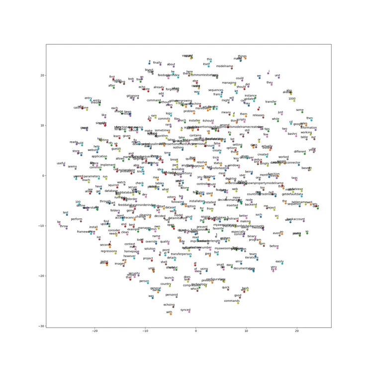
The word2vec example lets us visualize the result by reducing the dimension from a very large value (128 if you stick to default) to 2D. For information it uses a t-SNE algorithm, which is well-suited for visualizing high-dimensional data as it preserves as much as possible the relative distance between neighbours.

Here is the result I got:

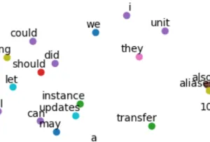
It is too dense to read, so see below an extract of what I got from my dataset:

We can see we have an area with pronouns in the top, and one with auxiliaries to the left.

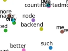
The relations highlighted just above were syntactic ones. On this other extract, we see semantic similarities:

The algorithm learned that node is a backend framework!

However with these few words, the model was not good enough to perform meaningful operations between vectors. I guess Theodoers need to write more blog articles to feed the word vectorization algorithm!

You can see below what word vectorization is capable of with this example coming from the Tensorflow page:

Conclusion

I hope that I managed in this article to share my enthusiasm for the rise of word vectorization and all the crazy applications that could ensue! If you are interested, I encourage you to look at papers that treat this subject more deeply:

• A more complete implementation example with Tensorflow
• You can also dive into this Kaggle competition that contains a lot of information about how to tackle a real use case